Natural Language UnderstandingStatistical Representation of Language and Knowledge

Natural Language
Understanding
Statistical Representation
of Language and Knowledge
Understanding
Statistical Representation
of Language and Knowledge
Mingming Sun
BIMSA
Outline

Outline
Why Statistical Representation
Vector Semantics for Word and Document
Topic Modeling
Neural Representations for Language
Neural Representations for Knowledge
1.3 Statistical Representation of Language and Knowledge 1.3.1 Why Statistical Representation
1.3 Statistical Representation of Language and Knowledge 1.3.1 Why Statistical Representation
Statistical Nature: Evolutionary Perspective
Statistical Nature: Evolutionary Perspective
As Natural Outcome of Language Emergence
Language is invented for maximizing information transition efficiency and reducing ambiguity.
So according to information theory, the human language naturally forms a certain distribution:
Zipf’s Law: The frequency of word usage in language follows a power-law distribution (a few words are used very frequently, while many words are used rarely), indicating a statistical regularity.
Menzerath’s Law: Longer linguistic units (e.g., sentences) tend to be composed of shorter components (e.g., words), which is also a statistical phenomenon.
Statistical Nature: Cognitive Perspective
Statistical Nature: Cognitive Perspective
Cognitive Perspective: Language Learning and Statistical Patterns
Child Language Acquisition: Studies show that infants use statistical learning abilities to identify phonetic patterns (such as word boundaries), indicating a strong link between language acquisition and statistical mechanisms.
Neuroscience: The brain utilizes probabilistic inference to predict the next word or sentence when processing language, a mechanism similar to modern neural language models (e.g., GPT).
Statistical Nature
Statistical Nature
The statistical nature of language is not an innate, a prior chacteristic but a natural property that gradually emerges during language evolution.
This statistical nature likely results from a combination of cognitive constraints, information transmission optimization, and biological evolution.
Statistical Representation vs Symbolic Representation
Statistical Representation vs Symbolic Representation
Symbolic Representation: Map Surface Form into Inner Symbolic Form with connection to real-world entities, facts, logics.
Statistical Representation: Find statistical connection between elements in the Surface Form, and connection to real-world may emerge.
1.3 Statistical Representation of Language and Knowledge 1.3.2 Vector Semantics for Words
1.3 Statistical Representation of Language and Knowledge 1.3.2 Vector Semantics for Words
What is Word: Recall the Structuralism
What is Word: Recall the Structuralism
A sign is the basic unit of meaning in language. It consists of:
Signifier (signifiant): The sound pattern or written form (e.g., the word “tree”).
Signified (signifié): The concept or meaning associated with the signifier (the mental image of a tree).
In N-Gram model, word is just surface strings (Signifier), and we do not directly care about its meaning (Signified).
We also talked about the logic representation of language, where the meaning of words is entity or relations.
Lets consider the meaning of word (Signified) more thoroughly.
Lemmas and Senses
Lemmas and Senses
Lemma is Signifier, and Sense can be considered some kind of Signified.
sense
mouse (N)
1. any of numerous small rodents...
2. a hand-operated device that controls a cursor...
1. any of numerous small rodents...
2. a hand-operated device that controls a cursor...
lemma
Modified from the online thesaurus WordNet
Relations: Synonymy
Relations: Synonymy
Synonyms have the same meaning in some or all contexts.
filbert / hazelnut
couch / sofa
big / large
automobile / car
vomit / throw up
water / H20
Relations: No Perfect Synonymy
Relations: No Perfect Synonymy
Note that there are probably no examples of perfect synonymy.
Even if many aspects of meaning are identical
Still may differ based on politeness, slang, register, genre, etc.
Examples:
water/H20: "H20" in a surfing guide?
big/large: my big sister != my large sister
The Linguistic Principle of Contrast
The Linguistic Principle of Contrast
Difference in form → difference in meaning
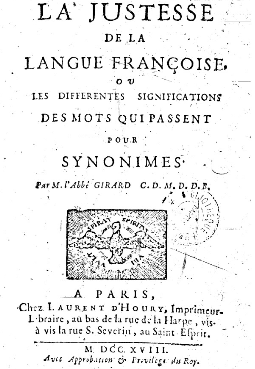
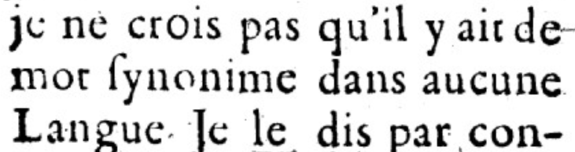
I do not believe that there is a synonymous word in any language
Relations: Similarity
Relations: Similarity
Not synonyms, but sharing some element of meaning
word1 | word2 | similarity |
vanish | disappear | 9.8 |
behave | obey | 7.3 |
belief | impression | 5.95 |
muscle | bone | 3.65 |
modest | flexible | 0.98 |
hole | agreement | 0.3 |
SimLex-999 dataset (Hill et al., 2015)
Relations: Antonymy
Relations: Antonymy
Senses that are opposites with respect to only one specific semantic feature, while they remain similar in other aspects.
For example:
hot vs. cold → Opposites in temperature, but both describe a degree of heat.
buy vs. sell → Opposites in perspective (buyer vs. seller), but both refer to the same transaction.
teacher vs. student → Opposites in role, but both exist within the context of education.
Relations: Relatedness
Relations: Relatedness
Words can be related in any way:
<coffee, tea>: similar; <coffee, cup>: related.
Semantic Field: Words that
cover a particular semantic domain
bear structured relations with each other.
Hospitals
surgeon, scalpel, nurse, hospital
Restaurants
waiter, menu, plate, food
Semantic Frame: Words that:
denote perspectives or participants in a particular type of event.
Buy :
buy, sell, goods
Travel
traveler, source, destination
Relations: Connotation(Sentiment)
Relations: Connotation(Sentiment)
Words have affective meanings
Positive connotations (happy, great, love)
Negative connotations (sad, terrible, hate)
Connotations can be subtle:
Positive connotation: copy, replica, reproduction
Negative connotation: fake, knockoff, forgery
Relations: Connotation(Sentiment)
Relations: Connotation(Sentiment)
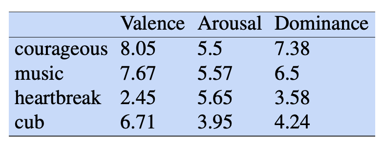
Words seem to vary along 3 affective dimensions(Osgood et al. (1957)):
valence: the pleasantness of the stimulus
arousal: the intensity of emotion provoked by the stimulus
dominance: the degree of control exerted by the stimulus
Summary: Senses and Relations
Summary: Senses and Relations
Senses (symbolic Signified)
Have a complex many-to-many association with words (Signifier)
Have relations with each other
Synonymy
Antonymy
Similarity
Relatedness
Connotation
The relation cannot be obtained from the sense through calculation.
The meaning of a word is its use in the language (Ludwig Wittgenstein)
The meaning of a word is its use in the language (Ludwig Wittgenstein)
Words are defined by their environments (the words around them)
If A and B have almost identical environments we say that they are synonyms. -- Zellig Harris (1954)
What does ongchoi mean?
What does ongchoi mean?
Suppose you see these sentences:
Ong choi is delicious sautéed with garlic.
Ong choi is superb over rice
Ong choi leaves with salty sauces
And you've also seen these:
…spinach sautéed with garlic over rice
Chard stems and leaves are delicious
Collard greens and other salty leafy greens
Conclusion:
Ongchoi is a leafy green like spinach, chard, or collard greens
Based on words like "leaves" and "delicious" and "sauteed"
ongchoi
ongchoi

Yamaguchi, Wikimedia Commons, public domain
空心菜
kangkong
rau muống
…
Basic Ideas
Basic Ideas
Idea 1: Defining meaning by linguistic distribution
Let's define the meaning of a word by its distribution in language use, meaning its neighboring words or grammatical environments.
Idea 2: Meaning as a point in multidimensional space
Defining meaning as a point in space based on distribution
Defining meaning as a point in space based on distribution
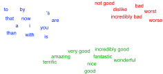
Each word = a vector (embedding) (not just "good" or "w45")
Similar words are "nearby in semantic space"
We build this space automatically by seeing which words are nearby in text
Vector Representation vs Symbolic Representation
Vector Representation vs Symbolic Representation
With words, a feature is a word identity
Feature 5: 'The previous word was "terrible"'
requires exact same word to be in training and test
With embeddings:
Feature is a word vector
'The previous word was vector [35,22,17…]
Now in the test set we might see a similar vector [34,21,14]
We can generalize to similar but unseen words!!!
Two kinds of embeddings
Two kinds of embeddings
Sparse Embedding
Representation calculated by explicit statistics of environments;
Dimension has explicit meaning;
Dense Embedding
Representation obtained by neural learning from environments;
Dimension generally has no explicit meaning.
From now on: Computing with meaning representationsinstead of string representations
From now on: Computing with meaning representations
instead of string representations
instead of string representations

1.3 Statistical Representation of Language and Knowledge 1.3.3 Sparse Embeddings
1.3 Statistical Representation of Language and Knowledge 1.3.3 Sparse Embeddings
The environment of words are documents;
Vector or distributional models of meaning are generally based on how words co-occur in documents;
We’ll look at two model methods: the word-document matrix and the word-word matrix.
Term-Document Matrix
Term-Document Matrix
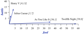
Each document is represented by a vector of words
Each word can be represented by a vector of documents


Visualizing document vectors
Visualizing document vectors
Word-word Matrix
Word-word Matrix
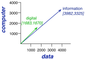
The count of word A co-occur with word B in a context range:
The whole document;
The limited window;


Visualizing word-word vectors
Visualizing word-word vectors
Raw frequency is a bad representation
Raw frequency is a bad representation
The co-occur frequency is the source of valuable information;
But overly frequent words like the, it, or they are not very informative about the context
It's a paradox! How can we balance these two conflicting constraints?
TF-IDF for Word-Document Representation
TF-IDF for Word-Document Representation
TF: Frequence of Term t in Document d
IDF: Inverse Document Frequence of Term t in Corpus
measure the importance of a word in the entire document collection D
TF-IDF:
If a word appears frequently in a document (high TF) but is relatively rare in the entire corpus (high IDF), then its importance in that document is greater.
Conversely, if a word is common across all documents (such as “the” or “is”), its IDF is low, resulting in a lower TF-IDF value.



PMI for Word-Word Representation
PMI for Word-Word Representation
PMI: (Pointwise mutual information)
It is a measure of how often two events x and y occur, compared with what we would expect if they were independent:
1.3 Statistical Representation of Language and Knowledge 1.3.4 Vector Semantics for Documents
1.3 Statistical Representation of Language and Knowledge 1.3.4 Vector Semantics for Documents
Let’s focus on Document
Let’s focus on Document
Could be a play or a Wikipedia article
But documents can be anything; even a paragraph can be considered a document.
However, we generally consider document to have complete and explicit meaning.
Bag of Words
Bag of Words
Recall the Word-Document Matrix:
Bag of Words (BOW): each document is represented by a vector of size with element of count/frequency.
TF-IDF Model
TF-IDF Model
TF-IDF: each document is represented by a vector of size with element of tf-idf value.

Applications of Document Embedding
Applications of Document Embedding
Text Classification
Used to train machine learning models (e.g., Naïve Bayes, SVM) for spam detection, sentiment analysis, and topic categorization.
Example: Detecting whether an email is spam based on the presence of certain words.
Text Clustering
Helps group similar documents together (e.g., k-means clustering).
Example: Categorizing news articles into topics like politics, sports, and entertainment.
Search Engine Ranking
Used to prioritize documents based on how uniquely relevant a term is.
Example: Google ranking a webpage higher if it contains unique words related to the search query.
Recommendation Systems
Measures similarity between documents using cosine similarity on TF-IDF vectors.
Example: Suggesting similar news articles based on the words in a given article.
Go deeper into Document Representation
Go deeper into Document Representation
One most fundamental attribute is Topics.
Recall the Synonymy and Semantic Field of word relatedness, words may be different but talking about the same topic;
Topic Similarity is an essential similarity of documents.
But BOW and TF-IDF do not represent the topic information.
How to model it?
Topics and Words
Topics and Words
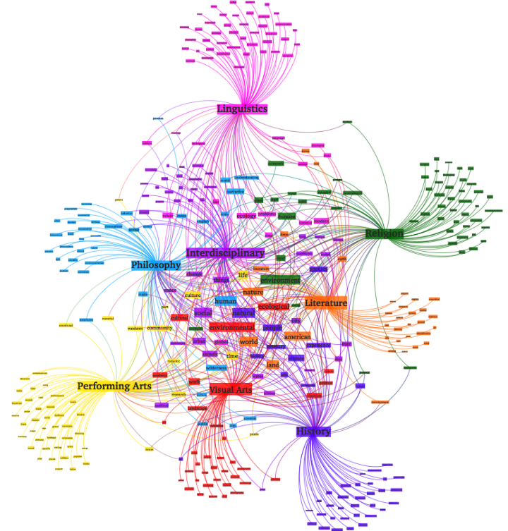
https://nanonets.com/blog/topic-modeling-with-lsa-plsa-lda-lda2vec/
Words are related by Semantic Field
Topic Modeling
Topic Modeling
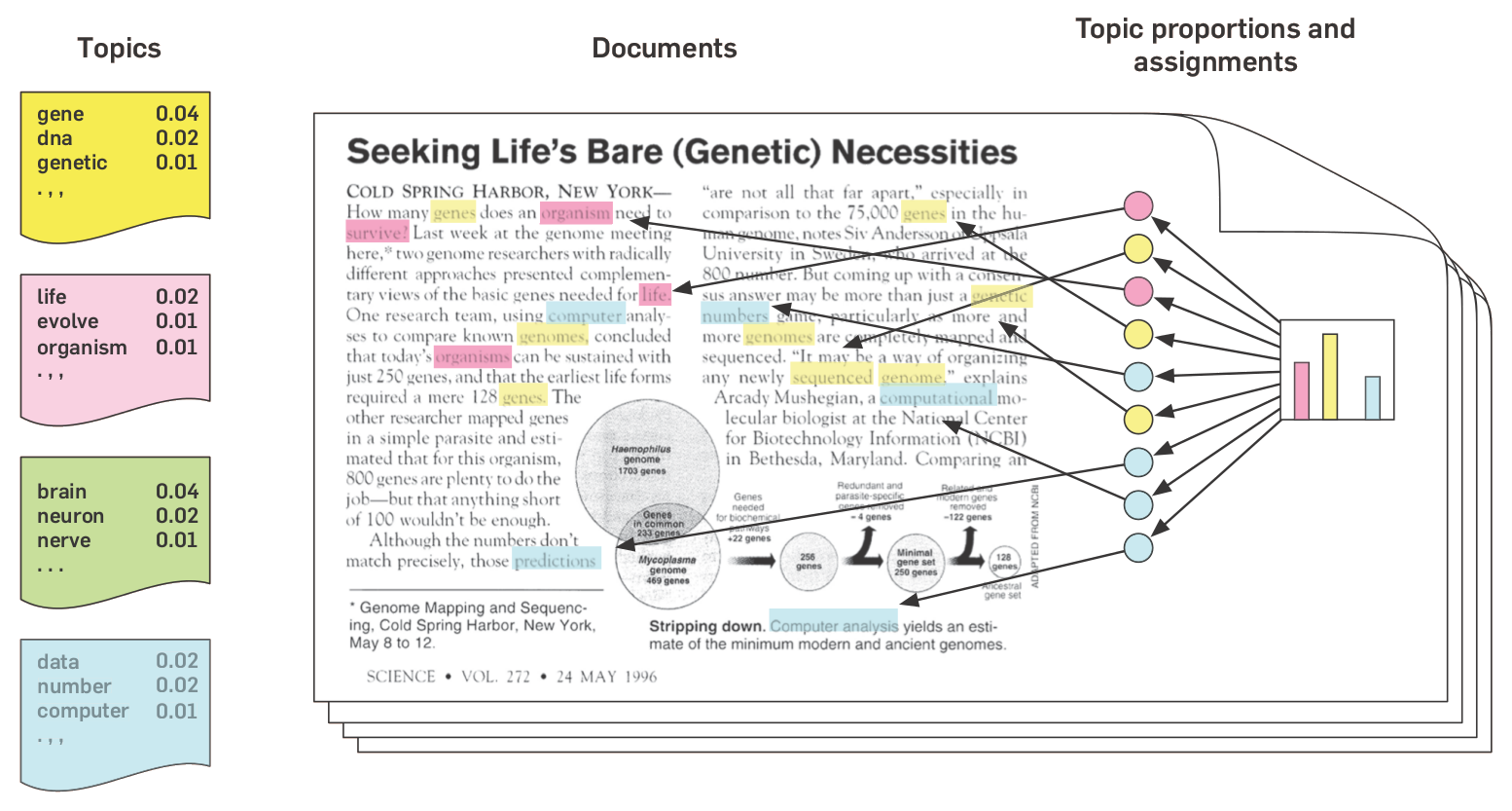
Key assumption:
each document consists of a mixture of topics, and
each topic consists of a collection of words.
The semantics of the document are governed by some “topics”;
We cannot observing the topics directly; It is hidden or “latent”;
The goal of topic modeling is to uncover these latent variables — topics — that shape the meaning of our document and corpus;
Latent Semantic Analysis (LSA)
Latent Semantic Analysis (LSA)
What we have: Documents and Terms (Words) Matrix (TF-IDF)
The matrix is very sparse, very noisy, and very redundant across its many dimensions;
Topics:
are hidden inner intermediate structures between the documents and words;
are with limited number, generally much smaller than that of doc and words.
How to discover the structures from the documents-words matrix?
Matrix Decomposition!
Latent Semantic Analysis (LSA)
Latent Semantic Analysis (LSA)
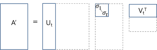
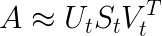
U ∈ ℝ^(m ⨉ t) emerges as our document-topic matrix,
V ∈ ℝ^(n ⨉ t) becomes our word-topic matrix.
S ∈ ℝ^(t ⨉ t) represents importance of a latent topic.
https://nanonets.com/blog/topic-modeling-with-lsa-plsa-lda-lda2vec/
Application of Topic related Embeddings
Application of Topic related Embeddings
With these document vectors and word vectors, we can now easily apply measures such as cosine similarity to evaluate:
the similarity of different documents
the similarity of different words
the similarity of terms (or “queries”) and documents (which becomes useful in information retrieval, when we want to retrieve passages most relevant to our search query).
Limitation of LSA
Limitation of LSA
Computationally Expensive
need for really large set of documents and vocabulary to get accurate results, where SVD is expensive for large-scale datasets;
Sensitivity to Noise and Parameter Selection
The choice of k (number of singular values retained) significantly impacts performance.
Lacks of Interpretation
We don’t know what the topics are (no modeling about topics).
Statistical Topic Modeling
Statistical Topic Modeling
Statistical View Point:
Document as a mixture of topics
Topic as a distribution over words;
Generative model for documents:
document features as being generated by sampling from the conditional probability of topic and words.
The goal of statistical topic modeling is to recover the distribution that best fit our observations -- document-term matrix.
Statistical Topic Modeling
Statistical Topic Modeling
Training on (large) corpus to learn:
Per-topic word distributions
Per-document topic distributions
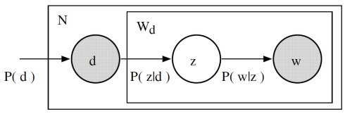
PLSA: Document Generation Procedure
PLSA: Document Generation Procedure
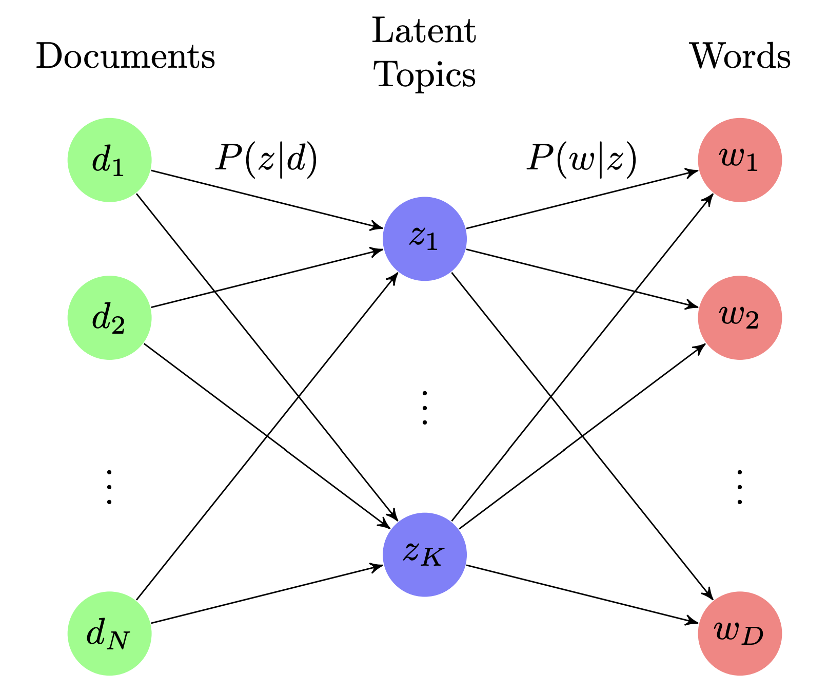
Document Generation Procedure:
Choose a document d from the document collection.
Select a topic z according to (each doc has a topic distribution, the parameter of PLSA).
Choose a word w according to (each topic has a word distribution, the parameter of PLSA).
Repeat steps 2 and 3 for each word in the document.
PLSA: Document, Topic, Words
PLSA: Document, Topic, Words
https://www.machinelearningplus.com/nlp/topic-modeling-visualization-how-to-present-results-lda-models/
PLSA
PLSA
https://homepages.inf.ed.ac.uk/rbf/CVonline/LOCAL_COPIES/AV1011/oneata.pdf
PLSA
PLSA
We want the model P(D,W) such that for any document d and word w, P(d,w) corresponds to that entry in the document-term matrix.
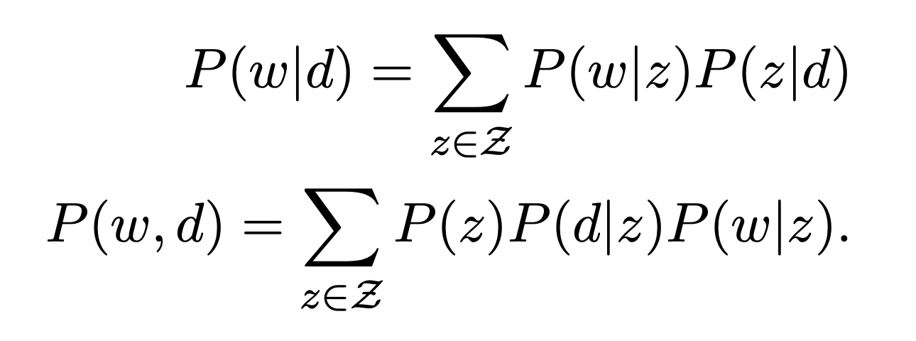
PLSA Training
PLSA Training
Joint probability model:
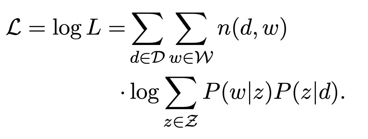
Likelihood

PLSA Training
PLSA Training
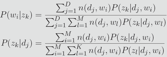
Training with EM:
Initialization of the per-topic word distributions and per-document topic distributions
E-step:
M-step:

PLSA and LSA
PLSA and LSA
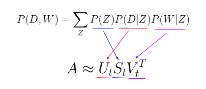
https://nanonets.com/blog/topic-modeling-with-lsa-plsa-lda-lda2vec/
Limitations of PLSA
Limitations of PLSA
No Generative Capability:
PLSA does not model how new, unseen documents are generated—it just assigns topics to existing documents.
Prone to Overfitting:
The number of parameters for PLSA is ;
Grows linearly with the number of documents.
Rarely used in practice.
Prior Distributions
Prior Distributions
If we have priors for the document-topic and word-topic distributions;
We can:
generate new document by sampling from the prior document-topic distribution;
reduced the number of parameter of the model to ;
Lending itself to better generalization.
The document-topic and word-topic distribution is multi-nominal;
What is the distribution of multi-nominal distribution?
Dirichlet Distribution
Dirichlet Distribution
The Dirichlet distribution is a probability distribution over the space of multinomial distributions:
to generate data X from a Dirichlet distribution with parameters ;
you first draw .
and then draw .

Explanation
Explanation
The overall distribution shape depends on the relative magnitudes of all ’s.
Relative magnitude determines the mean proportions: . A larger implies a higher expected proportion.
Absolute magnitude determines the degree of uncertainty: a larger leads to a more concentrated distribution, while a smaller leads to a more dispersed or sparse distribution
If all are small (<1) → The distribution is sparse, meaning most categories have near-zero probabilities, and only a few dominate.
If all are large (>1) → The distribution is dense, meaning all categories tend to have moderate values.
If values are imbalanced → Some categories (with larger values) are more dominant than others.
Example of Dirichlet Distribution
Example of Dirichlet Distribution
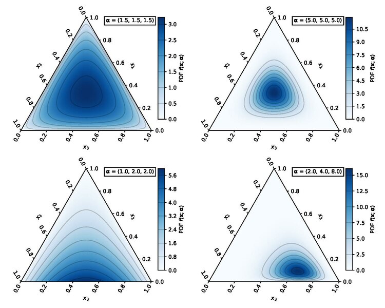
https://en.wikipedia.org/wiki/Dirichlet_distribution
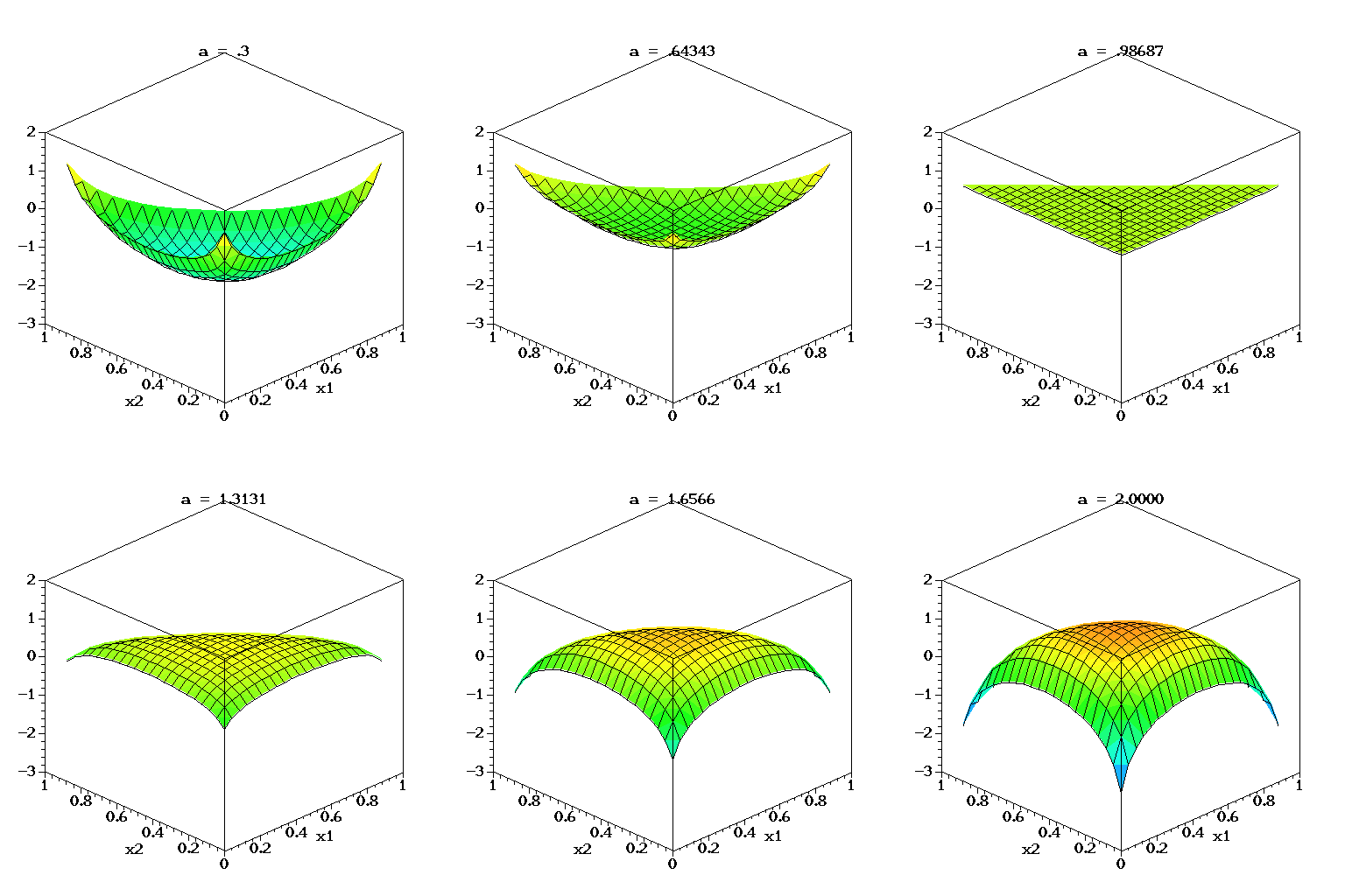
Latent Dirichlet Allocation
Latent Dirichlet Allocation
https://www.jmlr.org/papers/volume3/blei03a/blei03a.pdf
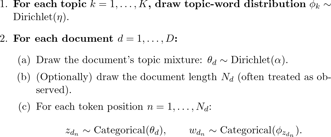
Latent Dirichlet Allocation
Latent Dirichlet Allocation
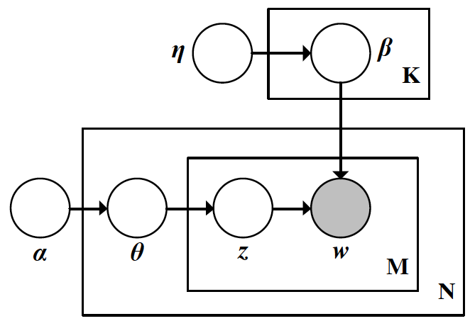
For each doc in a collection of N docs
For each word position in a doc of length M
Topic assignment to a word at position i in doc dj
Word token at position i in doc dj
Per-document topic distribution
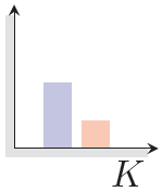
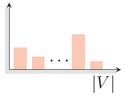
Per-topic word distribution
[Moens and Vulic, Tutorial @WSDM 2014]
Latent Dirichlet Allocation
Latent Dirichlet Allocation
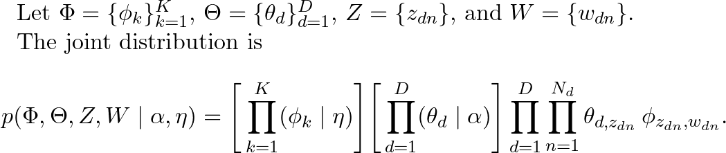
Parameter Estimation
Parameter Estimation
Given a corpus of documents , we are to find parameter and that maximize the log likelihood:
Can be solved by variational EM algorithm.
Inference
Inference
Given a document , we are to find the and .
Variational EM
Gibbs sampling
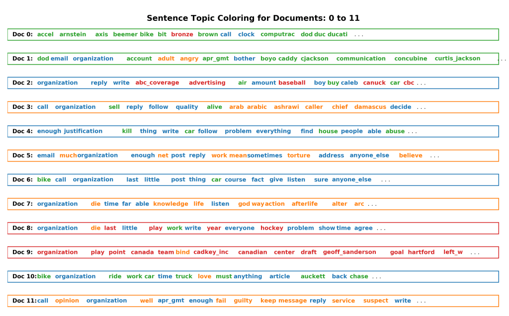
Case Analysis: LDA on News Data
Case Analysis: LDA on News Data
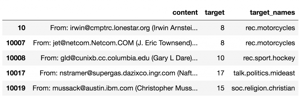
https://www.machinelearningplus.com/nlp/topic-modeling-visualization-how-to-present-results-lda-models/
Case Analysis: learned LDA Topics by Gensim
Case Analysis: learned LDA Topics by Gensim
https://www.machinelearningplus.com/nlp/topic-modeling-visualization-how-to-present-results-lda-models/
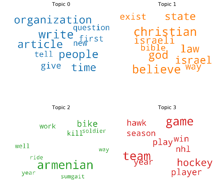
0, 0.017*"write" + 0.015*"people" + 0.014*"organization" + 0.014*"article" +
#> 0.013*"time" + 0.008*"give" + 0.008*"first" + 0.007*"tell" + 0.007*"new" +
#> 0.007*"question
1, 0.008*"christian" + 0.008*"believe" + 0.007*"god" + 0.007*"law" +
#> 0.006*"state" + 0.006*"israel" + 0.006*"israeli" + 0.005*"exist" +
#> 0.005*"way" + 0.004*"bible"
2, 0.024*"armenian" + 0.012*"bike" + 0.006*"kill" + 0.006*"work" +
#> 0.005*"well" + 0.005*"year" + 0.005*"sumgait" + 0.005*"soldier" +
#> 0.004*"way" + 0.004*"ride"
3 0.019*"team" + 0.019*"game" + 0.013*"hockey" + 0.010*"player" +
#> 0.009*"play" + 0.009*"win" + 0.009*"nhl" + 0.009*"year" + 0.009*"hawk" +
#> 0.009*"season"
Case Analysis: Top-N words cloud in Each Topic
Case Analysis: Top-N words cloud in Each Topic
Case Analysis: Dominant topic and its percentage contribution in each document
Case Analysis: Dominant topic and its percentage contribution in each document
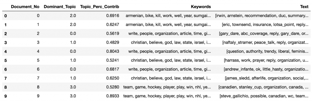
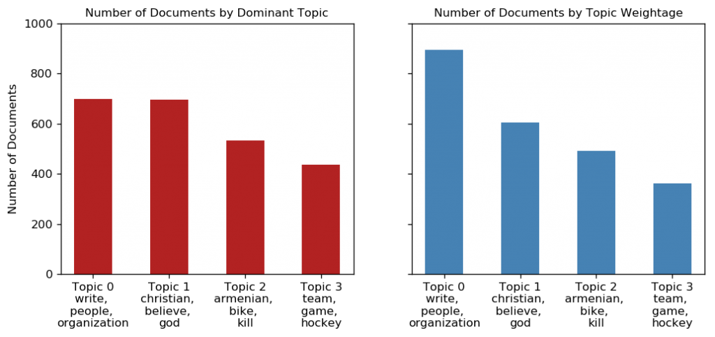
Case Analysis: Dominant topic and its percentage contribution in each document
Case Analysis: Dominant topic and its percentage contribution in each document
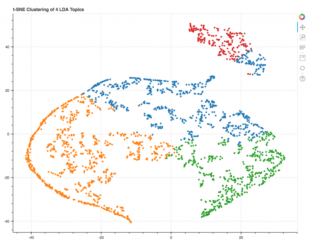
Case Analysis: t-SNE Visualization of Documents
Case Analysis: t-SNE Visualization of Documents
1.3 Statistical Representation of Language and Knowledge 1.3.5 Neural Embeddings
1.3 Statistical Representation of Language and Knowledge 1.3.5 Neural Embeddings
Relax the Constraint of Parametric Model
Relax the Constraint of Parametric Model
Parametric Models
A parametric model assumes a fixed number of parameters and a specific functional form (structure). The learning process involves estimating these parameters based on the given data.
Sparse Embeddings are Parametric Models:
TF-IDF, PMI, PLSA, LDA
Focus on objective, relax the capacity of models, let the data drive the direction of the model.
Learning Representation
Learning Representation
Recall: The meaning is determined by its environment, that is, neighborhood;
Words cooccur means their embeddings has certain relations.
How about predicting the neighborhood from the embedding?
Predicting each other: Word2Vec
Predicting the co-occurrence: GloVe
Word embeddings = the weights of learned machines.
Big idea: self-supervision by co-occurrence information without human label;
1.3 Statistical Representation of Language and Knowledge 1.3.6 Word2Vec
1.3 Statistical Representation of Language and Knowledge 1.3.6 Word2Vec
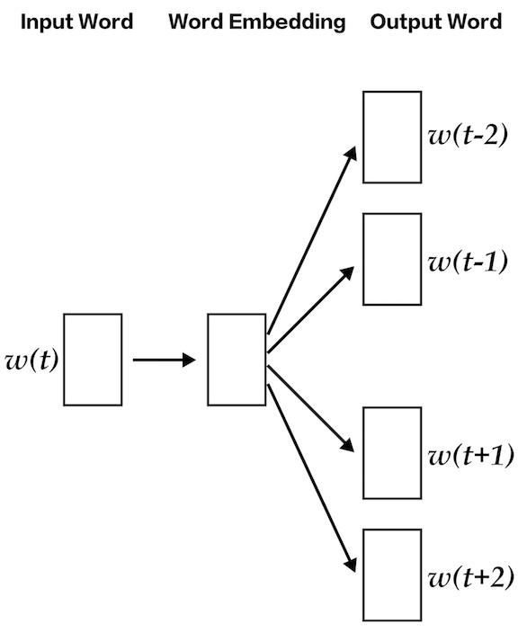
Word2Vec Overview
Word2Vec Overview
We have a large corpus (“body”) of text: a long list of words
Every word in a fixed vocabulary is represented by a vector
Go through each position t in the text, which has a center word c and context (“outside”) words o
Use the similarity of the word vectors for c and o to calculate the probability of o given c (or vice versa)
Keep adjusting the word vectors to maximize this probability
(Mikolov et al. 2013)
Skip-Gram: The context window
Skip-Gram: The context window
Assume a +/- 2 word window, given training sentence:
…lemon, a [tablespoon of apricot jam, a] pinch…
c1 c2 [target] c3 c4
Skip-Gram: Positive Samples
Skip-Gram: Positive Samples
Assume a +/- 2 word window, given training sentence:
…lemon, a [tablespoon of apricot jam, a] pinch…
c1 c2 [target] c3 c4

Skip-Gram: Negative Samples
Skip-Gram: Negative Samples
Assume a +/- 2 word window, given training sentence:
…lemon, a [tablespoon of apricot jam, a] pinch…
c1 c2 [target] c3 c4
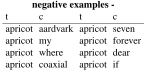
For each positive example we'll grab k negative examples, sampling by frequency
Skip-Gram: Negative Samples
Skip-Gram: Negative Samples
Assume a +/- 2 word window, given training sentence:
…lemon, a [tablespoon of apricot jam, a] pinch…
c1 c2 [target] c3 c4
Skip-Gram: Probabilities
Skip-Gram: Probabilities
Assume a +/- 2 word window, given training sentence:
Given a candidate (word, context) pair :
(apricot, jam)
(apricot, aardvark)
…
We want to compute the probability using their embeddings
…lemon, a [tablespoon of apricot jam, a] pinch…
c1 c2 [target] c3 c4
How to Compute 𝑃(+|𝑤, 𝑐)
How to Compute 𝑃(+|𝑤, 𝑐)
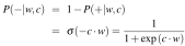
The probability of prediction should be definitely related to relatedness or similarity.
Two vectors are similar if they have a high dot product
Cosine is just a normalized dot product
So
𝑃(+|𝑤, 𝑐) can be obtained by normalize it to a probability.
For one context word: 𝑃(+|𝑤, 𝑐)
For one context word: 𝑃(+|𝑤, 𝑐)

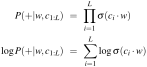
For the Full Context: 𝑃(+|𝑤, 𝑐1:𝐿)
For the Full Context:
We have lots of context words.
We'll assume independence and just multiply them:
The Parameters – Embeddings
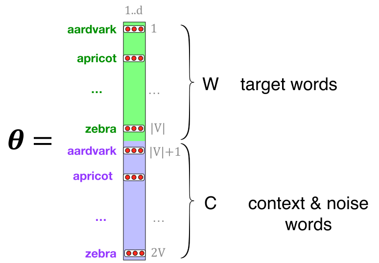
The Parameters -- Embeddings
Learning Procedure
Learning Procedure
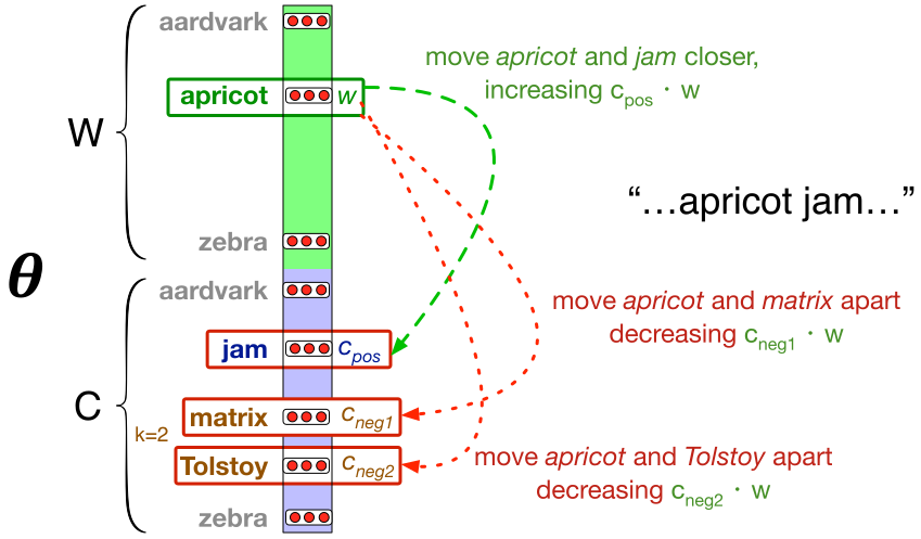
Given the set of positive and negative training instances, and an initial set of embedding vectors
The goal of learning is to adjust those word vectors such that we:
Maximize the similarity of the target word, context word pairs drawn from the positive data
Minimize the similarity of the pairs drawn from the negative data.
Loss Function
Loss Function
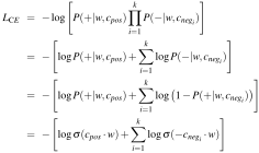
Maximize the similarity of the target with the actual context words, and minimize the similarity of the target with the k negative sampled non-neighbor words.
Optimization: Gradient Descent
Optimization: Gradient Descent
Gradients
Gradients
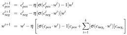
Start with randomly initialized C and W matrices, then incrementally do updates
Two representations?
Two representations?
Skip-Gram with Negative Sampling learns two sets of embeddings
Target embeddings matrix W
Context embedding matrix C
It's common to just add them together, representing word i as the vector
Learning Procedure Summary
Learning Procedure Summary
Start with random d-dimensional vectors as initial embeddings
Train a classifier based on embedding similarity
Take a corpus and take pairs of words that co-occur as positive examples
Take pairs of words that don't co-occur as negative examples
Train the classifier to distinguish these by slowly adjusting all the embeddings to improve the classifier performance
Throw away the classifier code and keep the embeddings.
Trained Word2Vec Embeddings
Trained Word2Vec Embeddings
Google Word2Vec: includes pre-trained vectors trained on a portion of the Google News dataset (consisting of about 100 billion words). The model contains 300-dimensional vectors for about 3 million words and phrases.
1.3 Statistical Representation of Language and Knowledge 1.3.7 GloVe
1.3 Statistical Representation of Language and Knowledge 1.3.7 GloVe
Glove: Basic Idea
Glove: Basic Idea
Word co-occurrence is the most important statistical information available for the model to ‘learn’. the word representation.
Glove: Use a Log-Bilinear (LBL) Regression Model to approximate the co-occurrence information:
the name of “Global”: Focus on the global co-occurrence information over the entire corpus.
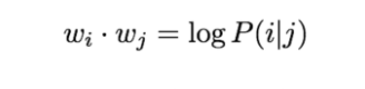
Why the Log-Bilinear Form?
Why the Log-Bilinear Form?
Let’s check the co-occurrence probability carefully.
Ratio of co-occur probabilities is more informative than the raw prob.
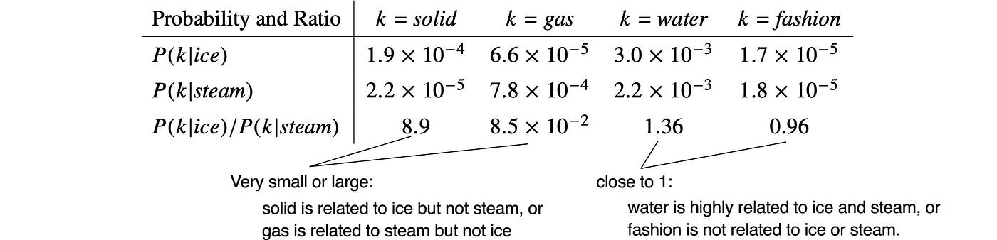
https://jonathan-hui.medium.com/nlp-word-embedding-glove-5e7f523999f6
Why the Log-Bilinear Form?
Why the Log-Bilinear Form?
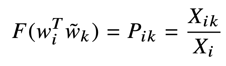
let us consider a function ‘F’ that models the ratio of probabilities relationship.


Add Linear Structure
Add Linear Structure
We want to given some desirable behavior for the embedding vector
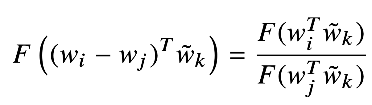
Linearity
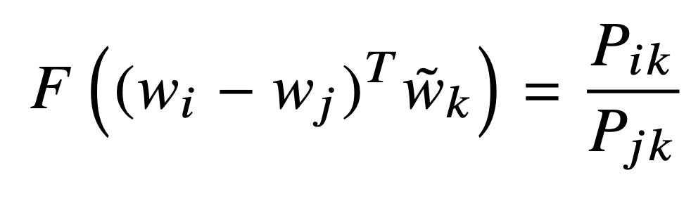
Add Symmetry between Words
Add Symmetry between Words
F be a homomorphism between the groups (R,+) and (R>0, ×),
Make it symmetry:


Loss: Weighting the co-occurrence
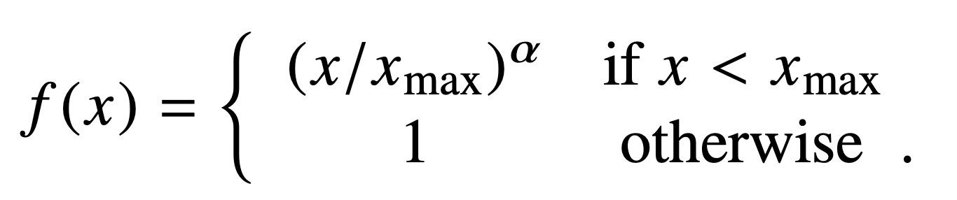
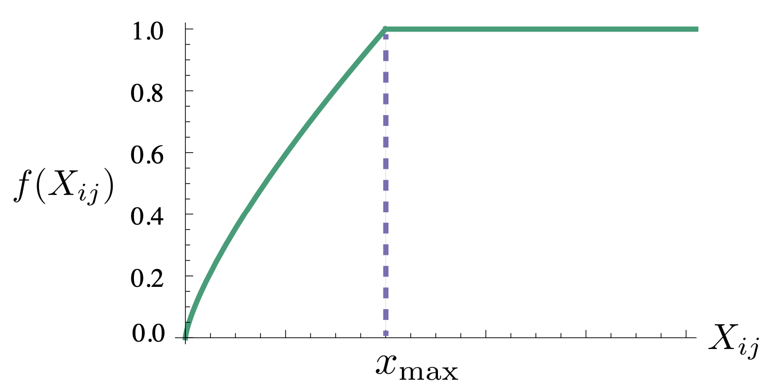
Loss: Weighting the co-occurrence
Large amount of rare cooccurrences are noisy and carry less information than the more frequent ones

https://nlp.stanford.edu/pubs/glove.pdf
Trained Glove Embeddings
Trained Glove Embeddings
Wikipedia 2014 + Gigaword 5 (6B tokens, 400K vocab, uncased, 50d, 100d, 200d, & 300d vectors, 822 MB)
Common Crawl (42B tokens, 1.9M vocab, uncased, 300d vectors, 1.75 GB)
Common Crawl (840B tokens, 2.2M vocab, cased, 300d vectors, 2.03 GB)
Twitter (2B tweets, 27B tokens, 1.2M vocab, uncased, 25d, 50d, 100d, & 200d vectors, 1.42 GB)
Available at: https://nlp.stanford.edu/projects/glove/
1.3 Statistical Representation of Language and Knowledge 1.3.8 Embedding Properties
1.3 Statistical Representation of Language and Knowledge 1.3.8 Embedding Properties
Relations
Relations
Small windows (C= +/- 2) : nearest words are syntactically similar words in same taxonomy
Hogwarts nearest neighbors are other fictional schools:
Sunnydale, Evernight, Blandings
Large windows (C= +/- 5) : nearest words are related words in same semantic field
Hogwarts nearest neighbors are Harry Potter world:
Dumbledore, half-blood, Malfoy
Example of Similarities
Example of Similarities
The neighbor of “Frog”
1.frogs 2. toad 3. litoria 4. leptodactylidae 5.rana 6. lizard 7.eleutherodactylus
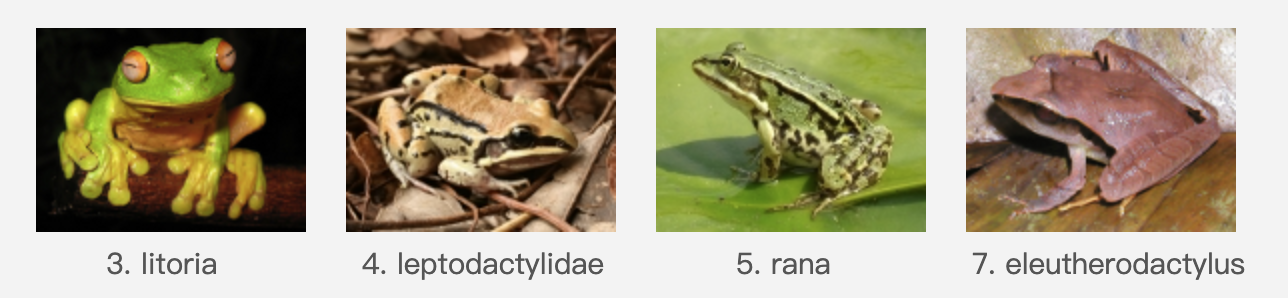
https://nlp.stanford.edu/projects/glove/
Analogical relations
Analogical relations
The classic parallelogram model of analogical reasoning (Rumelhart and Abrahamson 1973)
To solve: "apple is to tree as grape is to _____"
Add tree – apple to grape to get vine
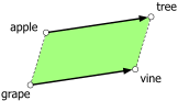
Analogical relations
Analogical relations
The parallelogram method can solve analogies with both sparse and dense embeddings (Turney and Littman 2005, Mikolov et al. 2013b)
is close to
is close to
For a problem , the parallelogram method is:

Structure in GloVE Embedding space
Structure in GloVE Embedding space
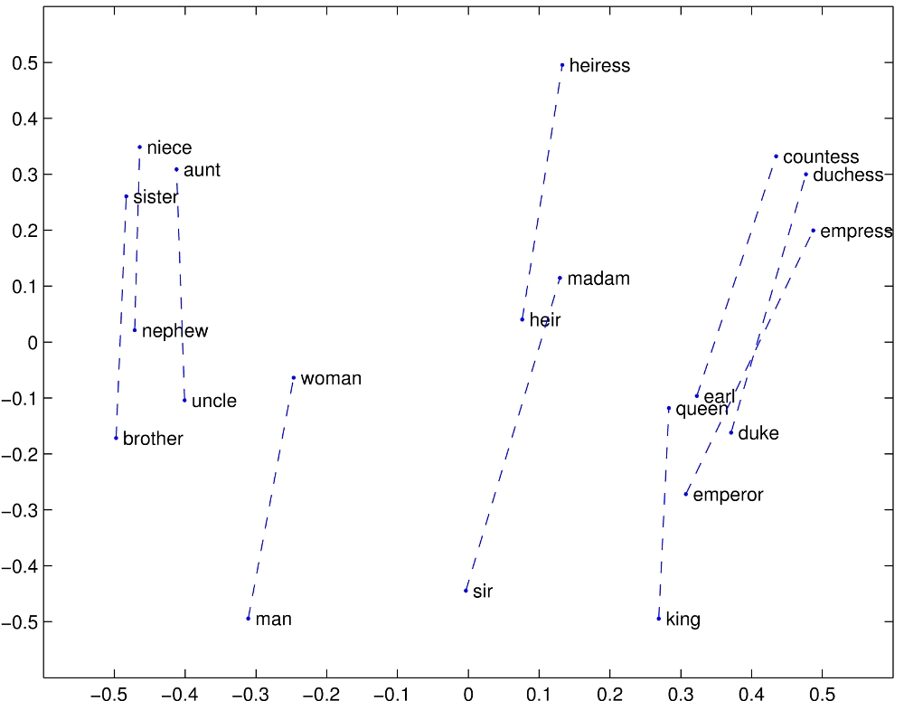
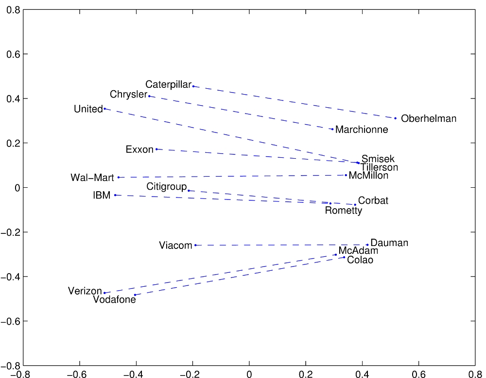
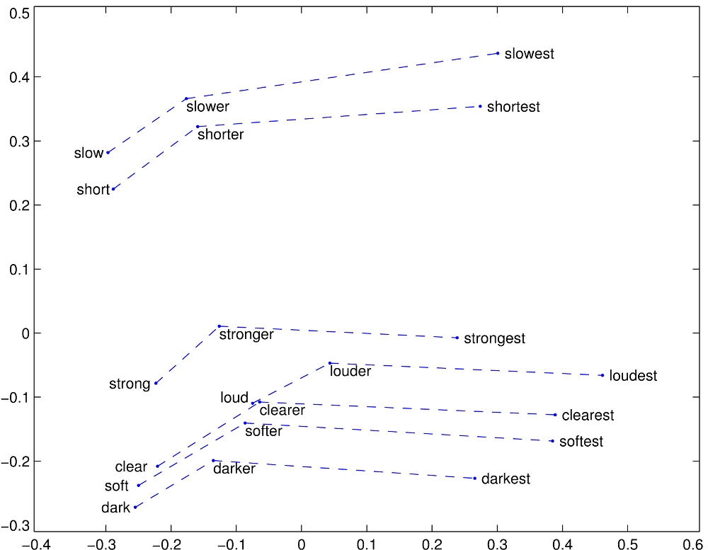
https://nlp.stanford.edu/projects/glove/
More about the Parallelogram Method
More about the Parallelogram Method
Parallelorgram method has been greatly developed and widely applied in the field of Knowledge Graph Embeddings (KGE).
It only seems to work for frequent words, small distances and certain relations (relating countries to capitals, or parts of speech), but not others. (Linzen 2016, Gladkova et al. 2016, Ethayarajh et al. 2019a)
Understanding analogy is an open area of research (Peterson et al. 2020)
Embeddings: a window onto Historical Semantics
Embeddings: a window onto Historical Semantics
Embeddings on different decades of historical text reveals meanings shift
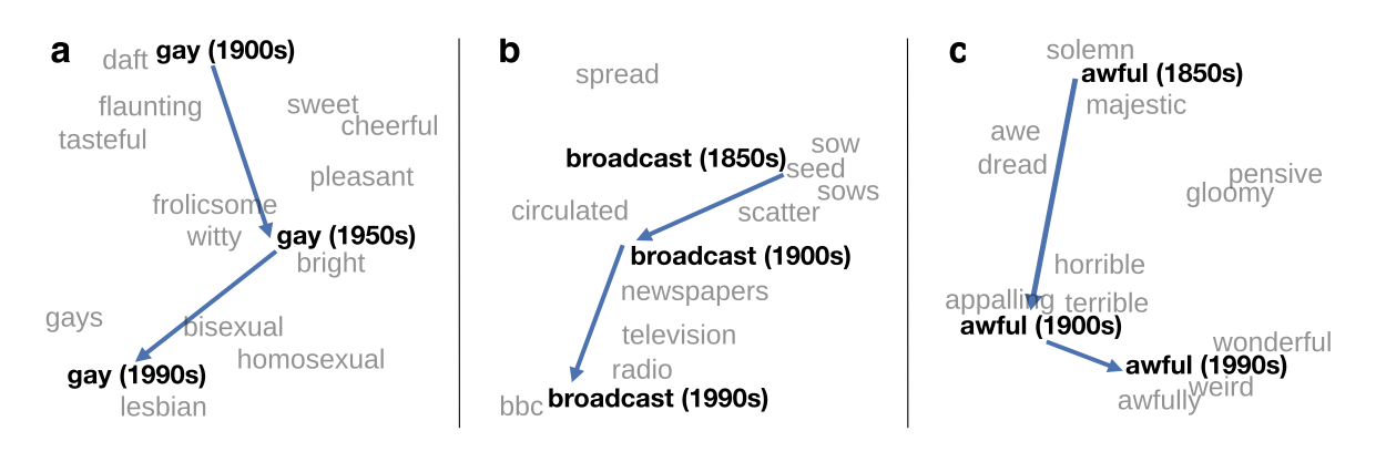
William L. Hamilton, Jure Leskovec, and Dan Jurafsky. 2016. Diachronic Word Embeddings Reveal Statistical Laws of Semantic Change. Proceedings of ACL.
Embeddings reflect cultural bias!
Embeddings reflect cultural bias!
Bolukbasi, Tolga, Kai-Wei Chang, James Y. Zou, Venkatesh Saligrama, and Adam T. Kalai. "Man is to computer programmer as woman is to homemaker? debiasing word embeddings." In NeurIPS, pp. 4349-4357. 2016.
Ask “Paris : France :: Tokyo : x”
x = Japan
Ask “father : doctor :: mother : x”
x = nurse
Ask “man : computer programmer :: woman : x”
x = homemaker
Algorithms that use embeddings as part of e.g., hiring searches for programmers, might lead to bias in hiring
Historical embedding as a tool to study cultural biases
Historical embedding as a tool to study cultural biases
Garg, N., Schiebinger, L., Jurafsky, D., and Zou, J. (2018). Word embeddings quantify 100 years of gender and ethnic stereotypes. Proceedings of the National Academy of Sciences 115(16), E3635–E3644.
Compute a gender or ethnic bias for each adjective: e.g., how much closer the adjective is to "woman" synonyms than "man" synonyms, or names of particular ethnicities
Embeddings for competence adjective (smart, wise, brilliant, resourceful, thoughtful, logical) are biased toward men, a bias slowly decreasing 1960-1990
Embeddings for dehumanizing adjectives (barbaric, monstrous, bizarre) were biased toward Asians in the 1930s, bias decreasing over the 20th century.
These match the results of old surveys done in the 1930s
1.3 Statistical Representation of Language and Knowledge 1.3.9 Knowledge Graph Embedding
1.3 Statistical Representation of Language and Knowledge 1.3.9 Knowledge Graph Embedding
Recall: Representation Learning
Recall: Representation Learning
Representation learning:
maps real-world objects into vectors (embeddings) in a vector space;
models their attributes, relationships, and interactions through the mathematical structure of these vectors;
thereby providing a computable and generalizable cognitive foundation for intelligent systems.
Can the elements (like relations) and operations (like reasoning) in KG be represented by embeddings?
Recall: Entity Linking
Recall: Entity Linking
We’ve learnt the entity embedding from its texture attributes.
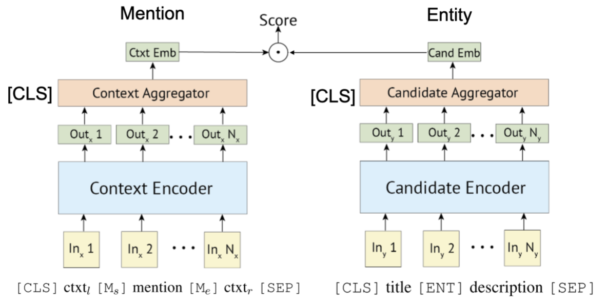
https://medium.com/nerd-for-tech/building-bi-encoder-based-entity-linking-system-with-transformer-6c111d86500
Node Embeddings
Node Embeddings
The meaning of nodes are defined by there environment.
To find embedding for nodes, just construct environment, and apply the Skip-Gram Algorithm.
DeepWalk
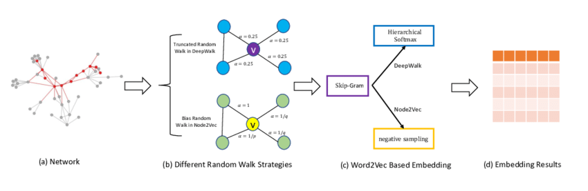
https://www.researchgate.net/figure/The-framework-of-DeepWalk-and-Node2Vec_fig2_343892685
Knowledge Graph Embeddings
Knowledge Graph Embeddings
Embeddings for KG elements:
Entity, Relation
How to obtain the embedding from the environment of KG?
What is the environments?
What is the objective of the embedding in this environment? That is, what is the expected relationship between the embedding of these elements?
Knowledge Graph Embeddings
Knowledge Graph Embeddings
Given a knowledge in KG , the entities and relations are logically connected;
Entity’s environments: associated relations and target entities;
Relation’s environments: associated head entities and tail entities.
We are expecting there exists certain relationship between their embeddings , that is .
Knowledge Graph Embedding
Knowledge Graph Embedding

https://arxiv.org/pdf/2410.14733
Recall: Analogical relations
Recall: Analogical relations
In word embedding:
is close to
is close to
For a problem , the parallelogram method is:
: a hidden relation representation?
Recall: Analogical relations
Recall: Analogical relations
https://nlp.stanford.edu/projects/glove/
Translation Based Embeddings
Translation Based Embeddings
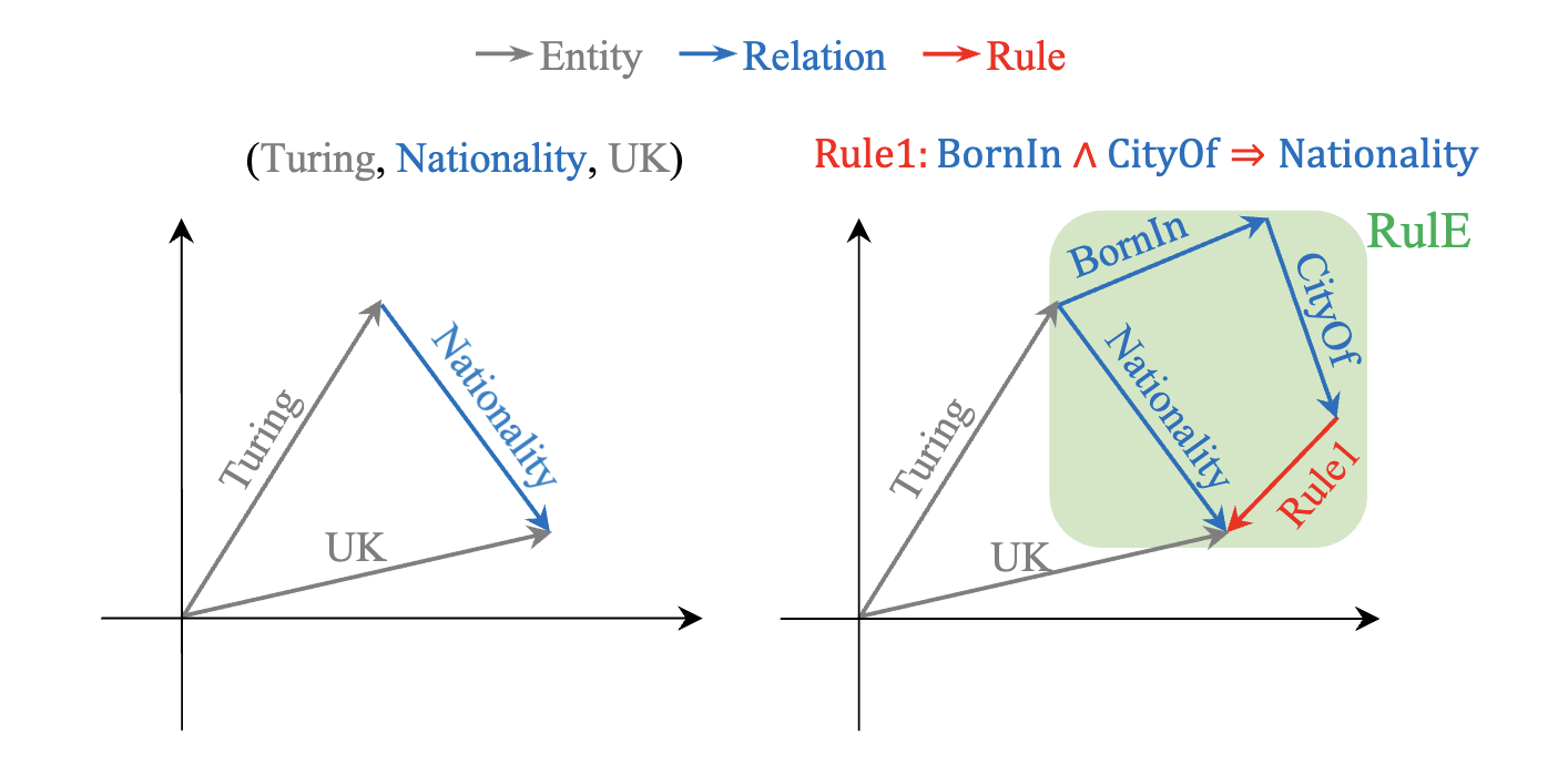
https://arxiv.org/pdf/2210.14905
TransE:
For positive facts, should be small;
For negative facts, should be large;
Training the Embedding Model
Training the Embedding Model
Use margin-based ranking loss:
For each positive triple (h, r, t), generate corrupted triple or by replace:
Head entity:
Tail entity:

Model Variants
Model Variants
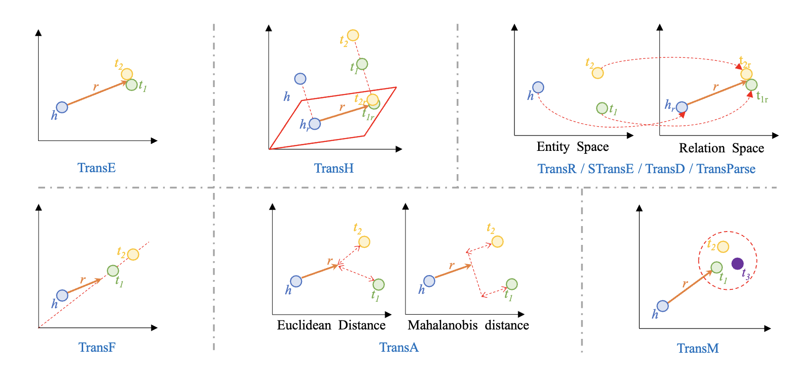
https://arxiv.org/pdf/2410.14733
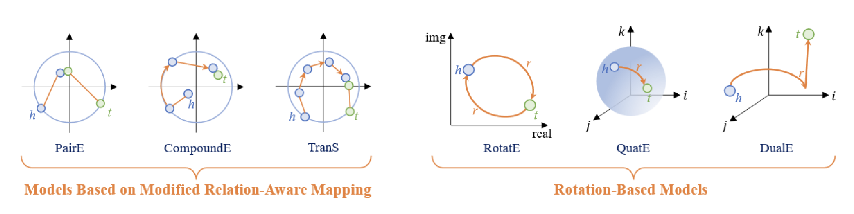
Model Variants
Model Variants
https://arxiv.org/pdf/2410.14733
Why so many variants?
Why so many variants?
https://arxiv.org/pdf/2410.14733
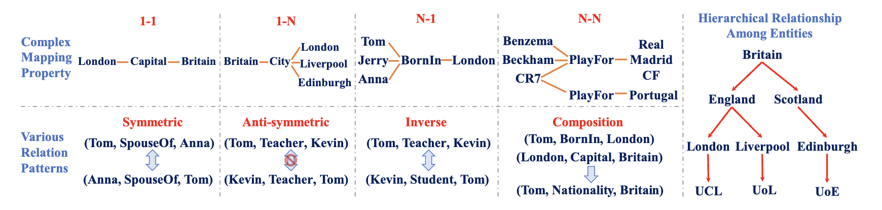
Why so many variants?
Why so many variants?
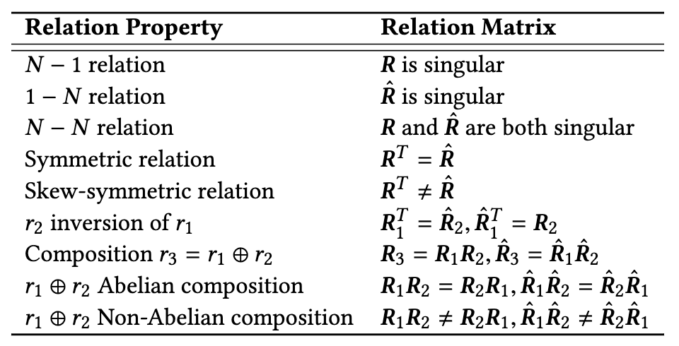
MQuadE
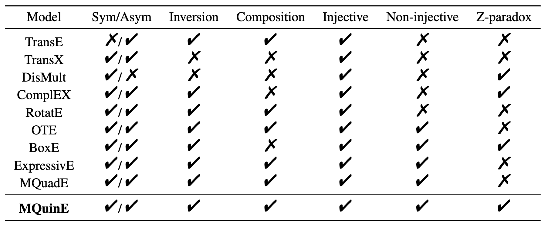
Why so many variants?
Why so many variants?
MQuinE
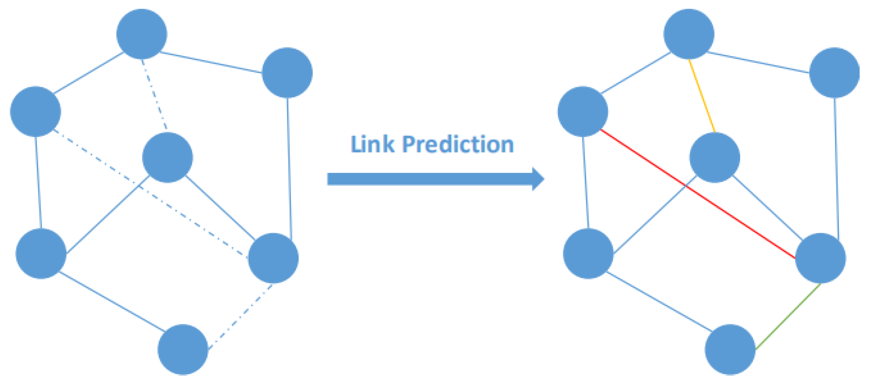
Applications of KGE
Applications of KGE
Link Prediction
or
Triplet Classification
is true or not
Entity Typing
Entity Matching
?
https://www.mdpi.com/2073-8994/13/3/485
1.3 Statistical Representation of Language and Knowledge 1.3.10 Suggested Readings
1.3 Statistical Representation of Language and Knowledge 1.3.10 Suggested Readings
Papers
Papers
1.3 Statistical Representation of Language and Knowledge 1.3.11 Assignment
1.3 Statistical Representation of Language and Knowledge 1.3.11 Assignment
Try and play with the ModelScope Platform
Try and play with the ModelScope Platform
Start the Jupyter Lab with CPU and GPU;
Make virtual environment;
Play with them, make sure the GPU is working as expected;
Remember to save data in the persistent path;
Remember to close the Jupyter Lab instance (Limited Time GPU)
The Report for Practical Project
The Report for Practical Project
Written in IPython notebook
A good experimental report: Introduction, Task description, Mathematical Model, Learning System Design, Experimental Setting, Model Selection, Performance Analysis and Case Study, Conclusion
Learning System Design: Write your math equation and implementation code and explanations
Experimental Setting: Describe your dataset, and hyper parameter candidates;
Model Selection: Perform cross-validation, choose the proper hyper-parameters and illustrate the underfit-overfit phenomenon;
Performance Analysis and Case Study: Evaluate the performance of the chosen model, and then analyze several good cases and bad cases.
Example: https://github.com/Sohaib1424/Support-Vector-Machine-from-scratch/blob/main/SVM.ipynb
Questions?
Questions?