3.3 Logic and Uncertainty 3.3.1 Natural Language to Logic: Formalization and Solving

3.3 Logic and Uncertainty 3.3.1 Natural Language to Logic: Formalization and Solving
Mingming Sun
BIMSA
BIMSA
Logic-LM: Formulation and Symbolic Solving
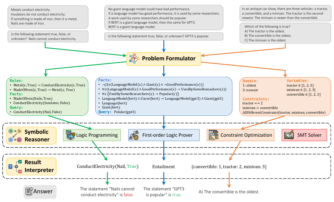
1. Problem formulator
The LLM uses in-context examples to generate task-specific symbols and constraints.
2. Symbolic reasoner
The CSP solver (python-constraint) returns
c=1,\quad t=2,\quad m=3.
3. Result interpreter
Map rank 1 back to the answer:
the convertible is oldest.
Logic-LM: Results and the Remaining Bottleneck
GPT-4 accuracy (%) · original Table 2 · no self-refinement
| Dataset | CoT | Logic-LM | Δ pp |
|---|---|---|---|
| PrOntoQA | 98.79 | 83.20 | −15.59 |
| ProofWriter | 68.11 | 79.66 | +11.55 |
| FOLIO | 70.58 | 78.92 | +8.34 |
| LogicalDeduction | 75.25 | 87.63 | +12.38 |
| AR-LSAT | 35.06 | 43.04 | +7.98 |
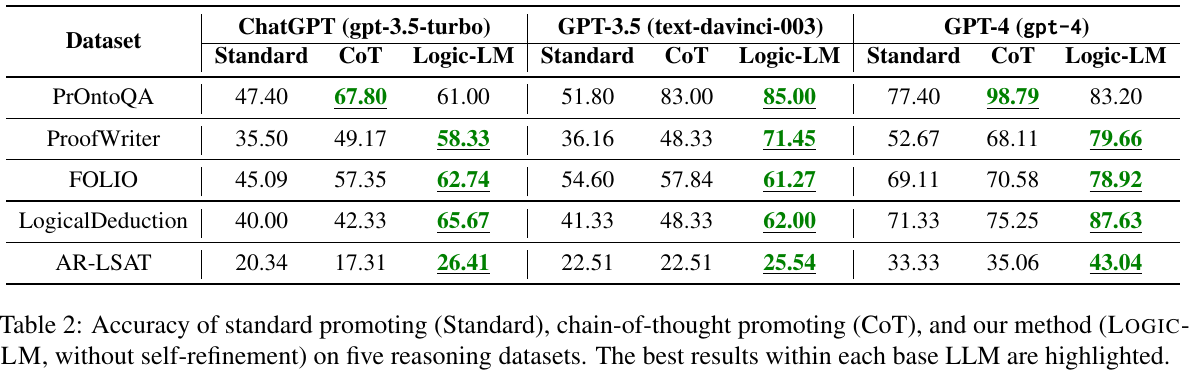
Protocol: same in-context examples; temperature 0. Non-executable cases fall back to CoT.
Finding: solver assistance helps many tasks, but can lose when formalization fails.
Separate refinement analysis (Table 3): GPT-4 FOLIO executable rate 79.9% → 85.8%; accuracy among executable cases 80.4% → 79.9%. These are different metrics.
LINC: Multiple Parses and Solver Votes
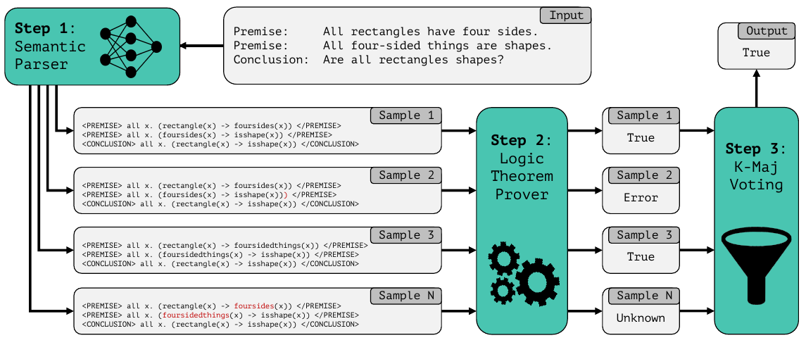
Four illustrated branches
Correct parse: True
Extra parenthesis: Error
Consistent renaming: True
Mismatched predicates: Unknown
Run Prover9 on each parse, then vote over valid labels.
Experiments use K=10. Shared translation errors can survive voting.
LINC: Strong Gains, with a Dataset Boundary
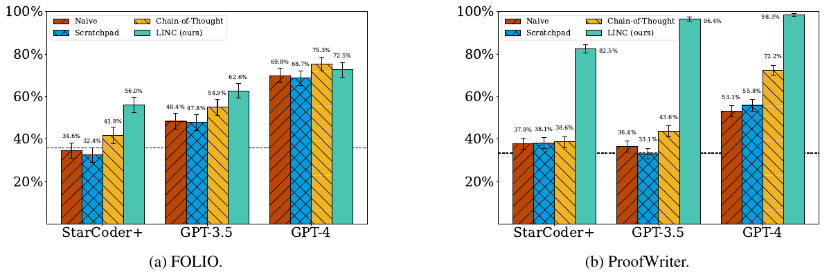
GPT-4 / ProofWriter:
CoT 72.2% → LINC 98.3% (+26.1 pp)
GPT-4 / FOLIO:
CoT 75.3% → LINC 72.5% (−2.8 pp)
FOLIO: 182 retained validation examples; ProofWriter: 360 balanced OWA examples. FOLIO difference is not significant (paper: p=0.58). Different subsets and voting protocols prevent direct comparison with Logic-LM’s table.
3.3 Logic and Uncertainty 3.3.2 Uncertain Evidence and Soft Rules

3.3 Logic and Uncertainty 3.3.2 Uncertain Evidence and Soft Rules
Errors, Conflicts and Missing Evidence
Errors, Conflicts and Missing Evidence
Reasoning systems combine facts and rules from documents, observations, and model predictions.
These inputs can contain errors, conflicts, and missing evidence.
We must assess evidence, reconcile constraints, and reason about unresolved facts.
Formal validity alone does not establish the reliability of the premises.
Logic and Probability: A Roadmap
Logic and Probability: A Roadmap
We will connect logical structure with uncertainty in evidence and rules:
Statistical Relational Learning
Markov Networks, Markov Logic, and Probabilistic Soft Logic
Statistical Relational Learning
Logic and Probability
Statistical Relational Learning
Statistical Relational Learning
Uncertainty in Evidence and Rules
Uncertainty in Evidence and Rules
Evidence extraction and interpretation involve uncertainty:
Arises during entity, relation, and event extraction
Common in instance matching/entity linking steps
Machine learning algorithms produce probabilistic outputs
Thresholding is often used to convert to hard labels
Heuristic or validation-based threshold tuning
Preserving Uncertainty for Joint Inference
Preserving Uncertainty for Joint Inference
Traditional practice: Discard uncertainty/Hard decision
New perspective: Leverage uncertainty as information
Example: Probabilistic extraction + ambiguous resolution ⇒ flag instance
Collective signals from multiple sources improve trust decisions
Cross-document or cross-task reinforcement
Cross-Algorithm and Cross-Task Challenges
Cross-Algorithm and Cross-Task Challenges
Uncertainty varies across algorithms
Some algorithms struggle where others succeed
Cross-task interactions:
e.g., Extraction vs. Instance Matching
Ensemble learning handles intra-task variation well
SRL needed to reason across tasks and dependencies
Structured Reasoning with SRL
Structured Reasoning with SRL
SRL offers a framework to handle:
Collective uncertainty
Domain expertise
Dependencies across evidence-processing stages
Helps integrate:
Domain-specific rules
Task-specific confidence levels
Output interdependencies
Dependencies Between Facts and Decisions
Dependencies Between Facts and Decisions
Local models often predict facts and decisions independently.
Shared evidence and domain rules create dependencies between these predictions.
Statistical Relational Learning (SRL) models these dependencies by integrating logic and probability.
Joint inference combines local evidence with these structured dependencies.
Modeling Dependencies
Modeling Dependencies
Relational dependencies are a key source of domain knowledge
Even simple ontologies (e.g., social networks) encode rich dependencies
Example relations: friendOf, spouseOf, votesFor
Domain rules derived from social science (e.g., spouses often vote alike)
From Intuition to Formal Rules
From Intuition to Formal Rules
Informal rules can be:
Spouses usually vote for the same candidate
Friends sometimes vote similarly
These are not deterministic — violations are allowed
SRL frameworks formalize such probabilistic dependencies
Formalizing with Weighted First-Order Logic
Formalizing with Weighted First-Order Logic
Rules are represented as weighted implications:
0.8: Spouse(A, B) ∧ VotesFor(A, P) → VotesFor(B, P)
0.1: Neighbors(A, B) ∧ VotesFor(A, P) → VotesFor(B, P)
0.4: Friends(A, B) ∧ VotesFor(A, P) → VotesFor(B, P)
Higher weight → stronger rule
Rules are soft constraints, not hard truths
Predicate Grounding and Domain Constraints
Predicate Grounding and Domain Constraints
Variables (A, B, P) must be grounded to real-world entities
Predicate constraints:
SRL supports expressing such structured domain knowledge robustly
Statistical Relational Learning Frameworks
Statistical Relational Learning Frameworks
Modern domains involve both:
Relational structure (dependencies between entities)
Uncertainty (confidence levels vary across rules)
Statistical learning handles uncertainty
Relational learning models structure
SRL unifies both approaches into a powerful framework
What SRL Enables
What SRL Enables
Core tasks supported by SRL:
Classification
Link prediction
Link-based clustering
Applications span social networks, recommender systems, knowledge graphs, etc.
SRL has become a feasible and promising research area due to advances in both statistical and relational learning
Key Requirements for an SRL Framework
Key Requirements for an SRL Framework
A successful SRL framework should:
Combine first-order logic with probabilistic graphical models
Support standard SRL tasks (e.g., link prediction, classification)
Allow incorporation of domain knowledge
Enable reuse and extension of methods from:
Statistical learning
Probabilistic and logical inference
Inductive logic programming
Weighted Logic and Probability
Weighted Logic and Probability
Markov Logic unifies probabilistic graphical models and first-order logic.
It is the Fundamental Model for SRL
It was proposed to meet a set of desiderata for probabilistic knowledge representation.
Before diving into MLNs, we first examine Markov Networks (also called Markov Random Fields).
Markov Random Fields
A Markov Network (also called a Markov Random Field, MRF) is an undirected graphical model.
It models the joint probability distribution of a set of random variables using a graph structure to encode their dependencies.
Key features:
Nodes represent variables
Edges represent direct probabilistic dependencies
Cliques define local compatibility functions
Conditional Independence in Markov Networks
Conditional Independence in Markov Networks
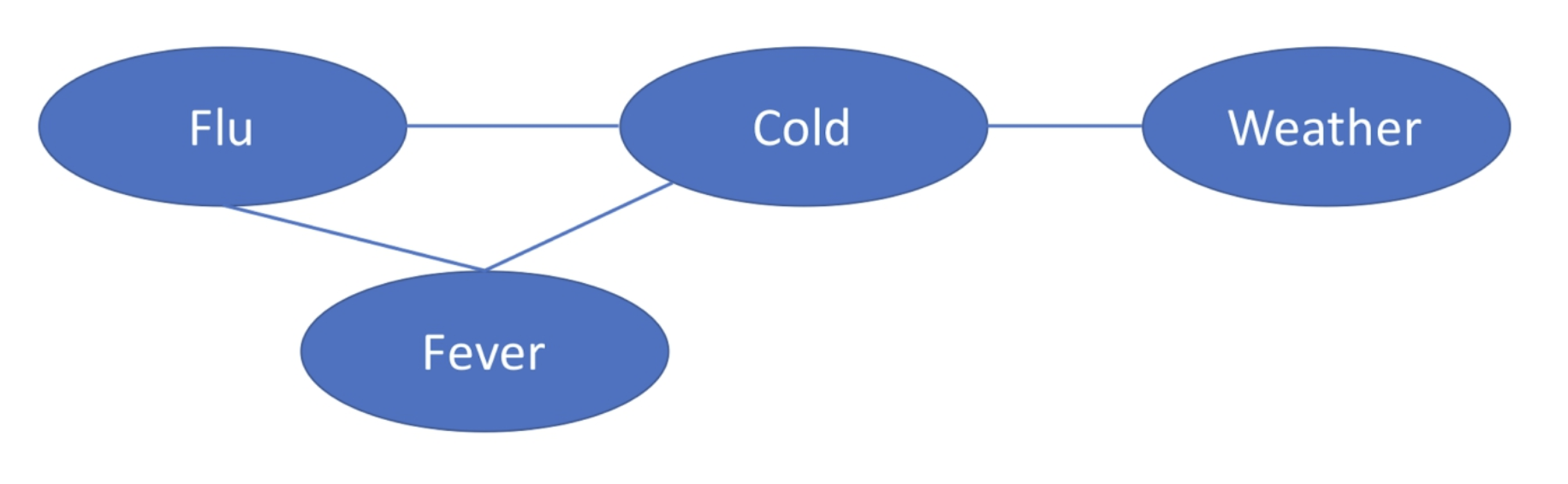
In an undirected graphical model, we aim to express the following form of conditional independence:
Each variable is only directly dependent on its neighbors; any influence from other variables is mediated through these neighbors.
To capture this locality, we need to define local structures in the graph that encode “energy” or “compatibility.”
These local structures are exactly the cliques — fully connected subsets of nodes where every pair is directly linked.
Conditional Independence: A Graph Example
Conditional Independence: A Graph Example
Clique Factorization and Hammersley–Clifford
Clique Factorization and Hammersley–Clifford
Hammersley-Clifford theorem:
For a joint probability distribution that satisfies certain conditions (e.g., being strictly positive), if it obeys the Markov properties implied by a graph, then it can be factorized as a product of potential functions over the cliques of the graph:
: Potential function defined over clique
: Value assignment to the variables in clique
: Normalization constant (partition function)
This result shows that only by defining potential functions over cliques can we fully capture the local dependencies encoded in the graph’s structure.

Log-Linear Models: Features and Weights
Log-Linear Models: Features and Weights
The potential function can be expressed by:
For example:
The probability can be expressed as log-linear models:
Each featureis a real-valued function (often binary)


A Two-Variable Markov Network
A Two-Variable Markov Network
A minimum Markov Network
Each is a boolean random variable
We define a potential function for this clique, which captures a certain preference or compatibility between and .

Potentials: Scoring Four Worlds
Potentials: Scoring Four Worlds
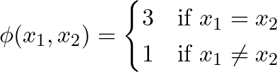
We hope the probability is larger when , so define:
0
|
0
|
3
|
0
|
1
|
1
|
1
|
0
|
1
|
1
|
1
|
3
|
Normalization, Marginals and MAP
Normalization, Marginals and MAP
Probability:
0
|
0
|
3/8
|
0
|
1
|
1/8
|
1
|
0
|
1/8
|
1
|
1
|
3/8
|


From Potentials to Features and Weights
From Potentials to Features and Weights
Define feature function :
Define potential function:
Let , then :
If
If
Potential function → Feature function + Weight


Feature Representation and Learnability
Feature Representation and Learnability
Avoid enumerating all states:
Potential functions typically assign a value to every possible state of a clique.
If a clique contains k binary variables, the total number of states is , meaning the potential function must store values.
Feature functions generalize through logical structure:
A feature function can be defined to activate under specific logical conditions (e.g., ).
Only a limited number of meaningful features need to be defined, rather than covering all combinations.
This is akin to using rules to compress the representation space.
Easier to learn and optimize:
Feature functions form a linear combination in the log-likelihood expression.
The objective function is convex, making it amenable to efficient optimization (e.g., using L-BFGS).
Markov Networks: Parameter Learning
Markov Networks: Parameter Learning
Learn the parameters (weights) of the model from data.
Two main learning tasks:
Structure learning: Learn the graph structure and features themselves
Parameter learning: Estimate weights of feature functions , given the graph structure and feature functions.
Challenges:
Parameter learning: the computation of Z need iterate all possible value of random variables;
Markov Networks: Inference Queries
Markov Networks: Inference Queries
Goal: Given a Markov Network and observations, compute:
Marginal probability:
Conditional probability:
MAP estimation: Find
Challenge: Requires summing or maximizing over exponentially many joint configurations.
Markov Logic Networks
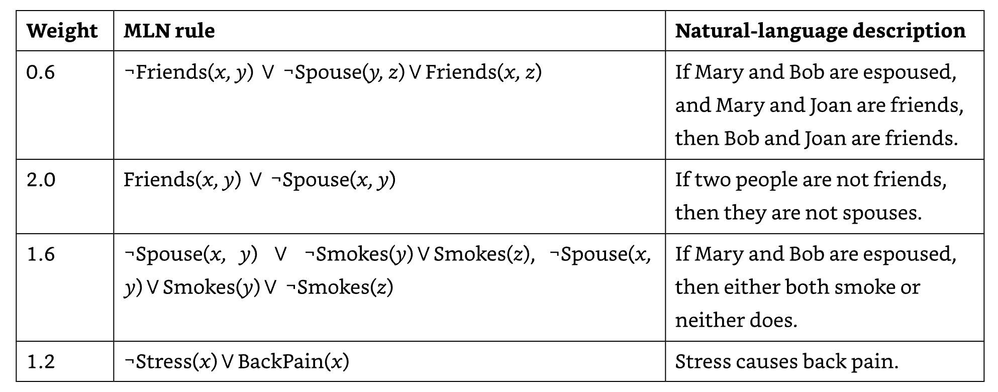
A Markov Logic Network is a set of pairs , where:
is a first-order logic formula
is a weight
This means: if a possible world satisfies a formula , it should be more probable; and the larger the weight , the higher the penalty for violating that formula.
MLN: Weighted Logical Rules
MLN: Weighted Logical Rules
MLN: From Templates to Networks
MLN: From Templates to Networks
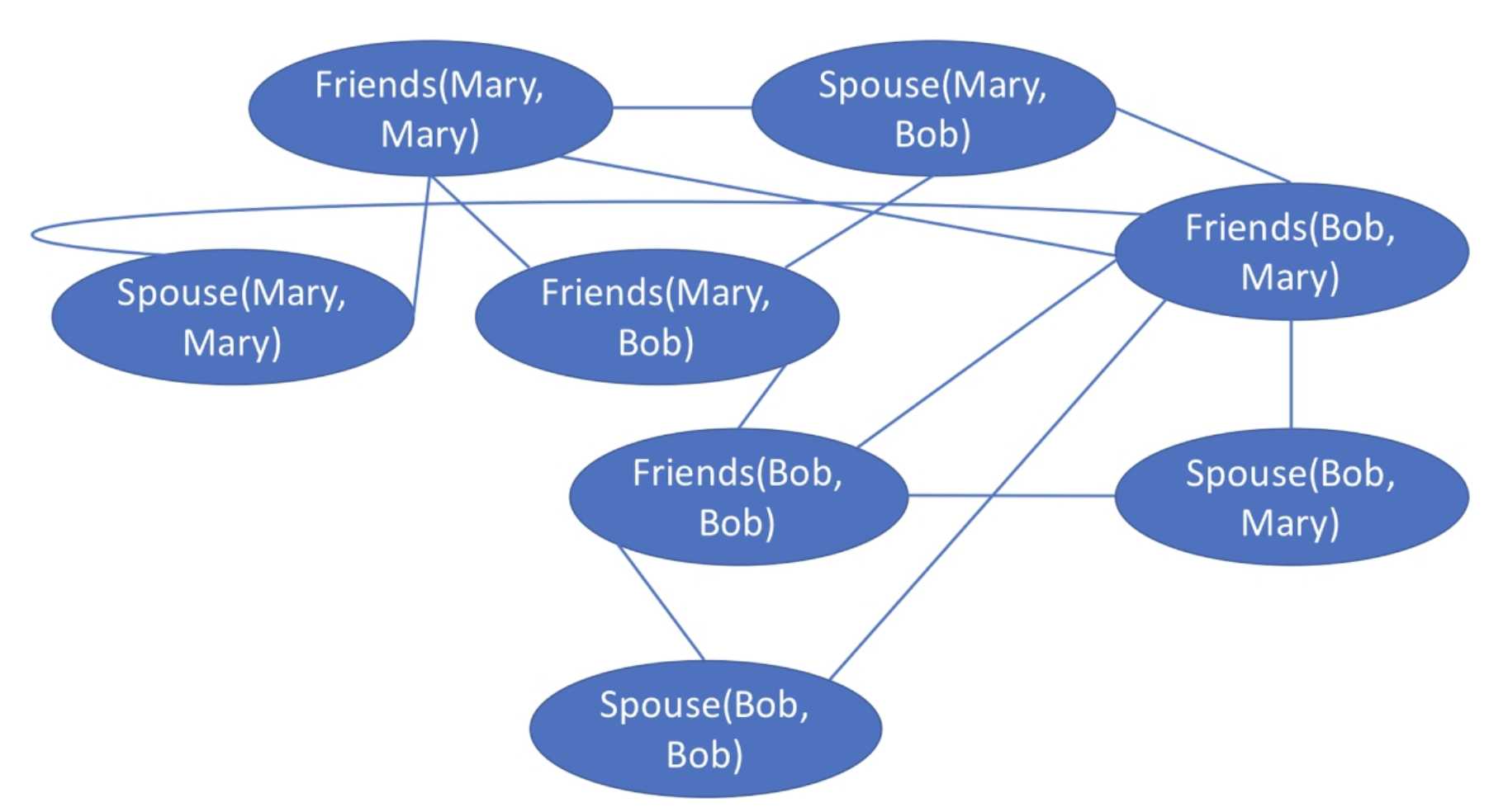
Generating Markov Network from MLN:
Given:
A set of rules
A set of Domain Constants
Steps:
Grounding: For each formula and the constant set, perform full grounding, i.e., enumerate all possible substitutions of variables with constants to generate specific ground clauses;
Making Cliques: Each grounded formula corresponds to a potential function, connecting all the variables (i.e., grounded Boolean predicates) involved in that formula;
Building the Network: All these variable nodes and potential functions together form a large undirected graph structure, which corresponds to the Markov Network.
MLN: Grounding with Typed Domains
MLN: Grounding with Typed Domains
Grounding is the process of replacing the variables in a first-order logic formula with concrete constants, thereby generating specific ground formulas (Boolean clauses).
Suppose you have the formula:
And your set of constants is:
Then the grounding process will generate all possible clauses, such as:
MLN: Ground Formulas as Factors
MLN: Ground Formulas as Factors
After grounding, a rule becoms
Each predicate (e.g., ) appearing in a ground formula becomes a variable node.
If multiple predicates appear in the same formula, they form a clique;
The feature function of the clique is defined as
is a possible world, i.e., a complete assignment of truth values to all predicate variables.
indicates whether the corresponding ground formula holds true in that world.

MLN: Shared Weights and World Probabilities
MLN: Shared Weights and World Probabilities
Connect all cliques into a huge network, and define the probability as:
Notice that feature functions grounded from a same rule share the same weights, so:
where is the times of rule been satisfied in the world .

MLN Example: Friends, Smoking and Cancer
MLN Example: Friends, Smoking and Cancer
MLN: Expressive Power and Hard Constraints
MLN: Expressive Power and Hard Constraints
General framework for probabilistic modeling:
Every probability distribution over discrete (or finite-precision numeric) variables can be represented as an MLN;
Unified Representation Framework:
unify symbolic and statistical approaches to knowledge representation
Compatibility with Other SRL Models
PRM, KBMC, SLP …
MLN: Inference and Learning Costs
MLN: Inference and Learning Costs
MLNs define a probability distribution over all possible worlds
Inference complexity
MAP is generally NP-hard; exact partition functions and marginals involve hard counting problems.
Learning expense:
Learning often requires inference or approximations;
Grounding Explosion:
Number of constants, Arity of predicates, Number of formulas
Probabilistic Soft Logic
PSL is a statistical relational learning framework that combines:
Logical rules
Probabilistic reasoning
Continuous-valued variables
Designed for efficient and scalable inference in real-world systems
“Soft logic + convex optimization for structured probabilistic reasoning”
PSL: Continuous Truth Semantics
PSL: Continuous Truth Semantics
Let a = v(A), b = v(B) ∈ [0, 1]. The last column uses a = 0.8, b = 0.6.
| Operation | Truth value | Logical meaning | Ex. |
|---|---|---|---|
| ⊥ Falsity | 0 | Always false. | 0 |
| ⊤ Truth | 1 | Always true. | 1 |
| ¬A Negation | 1 − a | “Not A”: the complement of A’s truth degree. | 0.2 |
| A ⇒ B Implication | min(1, 1 − a + b) | “If A, then B”: fully true when a ≤ b. | 0.8 |
| A ∨ B Weak OR | max(a, b) | “A or B”: take the larger truth degree. | 0.8 |
| A ∧ B Weak AND | min(a, b) | “A and B”: take the smaller truth degree. | 0.6 |
| A ⇔ B Equivalence | 1 − |a − b| | Both implications hold; fully true when a = b. | 0.8 |
| A ⊕ B Strong OR | min(1, a + b) | “A or B”: add truth degrees, capped at 1. | 1 |
| A ⊙ B Strong AND | max(0, a + b − 1) | “A and B”: subtract both shortfalls from 1, floor at 0. | 0.4 |
| A ⊖ B Difference | max(0, a − b) | A ⊙ ¬B: how much A exceeds B; violation of A ⇒ B. | 0.2 |
PSL rule AND/OR use the strong operations ⊙/⊕, usually written ∧/∨ in PSL.
The weak min/max rows are included for comparison; ⊕ here does not mean XOR.
PSL: Hinge-Loss Potentials and MAP
PSL: Hinge-Loss Potentials and MAP
1. Rule truth: A ⇒ B is ¬A ⊕ B, using Łukasiewicz strong OR.
t = v(A ⇒ B) = min(1, (1 − a) + b)
2. Violation is the shortfall from full truth: d = 1 − t.
d = 1 − min(1, 1 − a + b) = max(0, a − b)
a ≤ b: fully satisfied, d = 0.
Example: a = 0.6, b = 0.8 → d = 0.
a > b: penalize the gap, d = a − b.
Example: a = 0.8, b = 0.6 → d = 0.2.
3. Multiple premises: for A ⊙ B ⇒ C, let c = v(C).
L = max(0, a + b − 1), d = max(0, L − c) = max(0, a + b − c − 1)
4. Weighted loss and MAP: φi(x) = di(x)p, minimize Σi wiφi(x).
x ∈ [0, 1]n; observed values fixed. Nonnegative wi, p ∈ {1, 2}, affine hinges
and a convex feasible set give convex MAP inference. Soft truth is not P(B | A).
PSL: Learning Rule Weights
PSL: Learning Rule Weights
Input: A set of PSL rules and ground truth predicate values (training data)
Initialize weights: Typically set to 1.0 or randomly
Iterate:
Perform inference using the current weights
Compare the predicted values with the labeled data
Compute the loss and update the weights
Output: The learned optimal weight parameters
